SAXS Calibrants

A. C. Finnefrock

Jan 25, 2000
version 0.2

1  Introduction

SAXS (small-angle x-ray scattering) calibrants are used to accurately determine the sample-to-detector distance, which allows one to compute q (reciprocal-space lengths) for the image on an area detector. This document should help you understand how to find and use the various x-ray calibrants available in the laboratory, or make your own.

The essential criteria for any good calibrant are good reproducibility among samples, reasonably strong (intense) scattering, an appropriate length scale, and several orders of diffraction (a well-ordered sample). Broadly speaking, there are two types of calibrants: those that rely on a periodic structure in the calibrant, and those that exploit the geometrical form factor of the calibrant's constituents. These are discussed in turn.

2  Periodic Calibrants

Periodic calibrants are the traditional choice. In the laboratory, we use two types available immediately: silver stearate (d = 48.68 Å) and silver behenate [1,2] (d = 58.376 Å). For larger d-spacings, a common biophysical standard is rat collagen. The lattice constant d is given variously in the literature as 668 Å - 670 Å. (The former number is Eric Eikenberry's value.)

The silver stearate and silver behenate calibrants are easy to prepare. Fill a capillary at least 1 cm tall with the dry powder and seal it. (Flame sealing is easiest in this case, although the powder will burn if you do not leave at least little space). These samples must be stored in light-tight containers since they will slowly photodegrade. One solution is to wrap a test tube in black electrical tape and store the capillary within. To make the specimen to detector distance more precise, place a 0.1 or 0.2 mm filled capillary within a 1.0 or 1.5 mm capillary. Silver stearate and silver behenate are strong scatterers, so there will still be a sufficient signal.

The rat collagen is more difficult, and considerably more gruesome. (Eric Eikenberry is the expert on this protocol). Take a pair of dull wire cutters and snip a fresh rat tail 3/4 of the way through. Strip out the tendons and drop them into a petri dish containing a standard physiological buffer. The buffer should consist of 20 mM phosphate (pH 7.4) and 150 mM sodium chloride. Keep the tendons wet. Once dry, they will not rehydrate fully, leading to an irreproducible length scale in the range 620 Å to 650 Å.

The tendons are sticky threads which can be threaded through an open (acid-washed) capillary with some difficulty. Be sure to add buffer before sealing the capillary. Because this is animal tissue, the sample will only stay fresh a few days.

2.1  Theory

To calibrate an image, it is sufficient to know the specimen-to-phosphor distance z and the x-ray wavelength l.

An x-ray diffraction image from periodic calibrants exhibits Bragg scattering peaks centered at q given by Bragg's law,

n l = 2 d sinq

(1)

where d is the lattice spacing mentioned previously. The x-ray scattering vector q = k_f - k_i, has a length

q = 2 k sinq = 4 p l sinq

(2)

as shown in figure 1(a). Then (1) is more simply written

q d = 2 pn   .

(3)

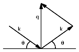
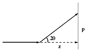
An x-ray diffracted through 2q will strike the detector (phosphor screen or image plate) at a distance p from the center. As shown in figure 1(b),

tan2 q = p z

(4)

where z is the sample-to-detector distance.

Approximating q » sinq » tanq and equating q in (2) and (4),

q = 2 pp lz   .

(5)

Thus from the wavelength l and the sample-to-detector distance z, q can be calculated for any transverse length p along the detector. (For Cu Ka radiation, l = 1.54 Å.)

This procedure for calibrating an image (given z and l) can be reversed to determine z (given a calibrant of known d and l). Combining (2) and (5),

z = p d n l   .

(6)

The peaks occur at positions p. Fitting these positions to a straight line, the slope then yields z directly. This same procedure is used by TV6, as described in the next section.

To test the validity of the small-angle approximation, consider silver stearate. This has the smallest d-spacing and hence the largest angle per diffraction order. If you used only the n = 10 diffraction peak and the small-angle approximation, you would compute d = 48.4755 Å instead of d = 48.68Å (a relative error of 0.4%). In general, you would use all visible orders n = 1,2, ¼, 10, so the error would be considerably less. Even in this case the error in z will be small. In contrast, the n = 10 diffraction peak for rat collagen produces only a 0.002% relative error by the small-angle approximation.

2.2  Software

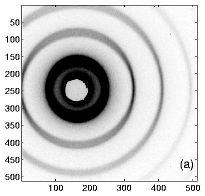
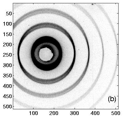
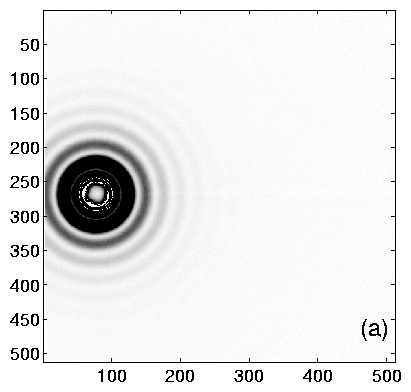
Using TV6, the procedure is as follows. Collect an diffraction image from the calibrant. The ideal image will have many orders of diffraction, with both (left and right) first-order peaks visible. Having at least one order on each side of the center helps to determine the q = 0 point accurately. Example images are shown in figure 2, and integrated profiles in figure 3.

Figure 2: Intensity maps of (a) silver stearate, (b) silver behenate.

After creating an intensity profile with dens, enter peak. Select the peaks by moving the mouse and entering numbers corresponding to the diffraction order. Press c to calibrate, and d to find the spec-to-phos distance. Enter the calibration length. You can check this calibration by fitting with f and regraphing with g, then showing tick marks with t. Record z, the spec-to-phos distance in pixels. This enables you to recreate the calibration later without repeating all of these steps.

Alernatively, you can do this in Matlab. In TV6, save your data as an rfile; this can be read by Matlab. Assuming the name of your rfile is rfilename.rf:

>> [x,y] = read_rfile('rfilename.rf');

>> qt_slice(x,y)

Then, choose Calibration -> Define calibration and answer the prompts. This defines a calibration by determining z given the l you enter. You can then calibrate this same image by choosing Calibration -> Calibrate or select another image first (File -> Load).

3  Spherical Calibrants

3.1  Materials

At present, four containers of spherical calibrants are available. First are polystyrene spheres from Duke Scientific (3050A) of radii 25 nm ± 1.0 nm and 1% concentration. Also from Duke Scientific (5020A) are larger spheres of radii 101.5 nm ± 2.2 nm and 10% concentration. Rudolf Sprik generously gave us two vials of silica spheres. The one labelled mEC1 is of radii of 27.8 nm ± 0.4 nm, while the mESiJ3-113 has nominal radii of 136 nm.

3.1.1  Procedures

The procedure for handling the colloidal suspensions, as given by Duke Scientific:

``For ease of use, these standards are packages in an aqueous suspension. They must be thoroughly dispersed in the bottle to assure statistically consistent samples. Allow the contents to come to room temperature before use. To disperse the particles, gently invert the bottle several times, then immerse in a low power ultrasonic bath (30 seconds). Do not shake the bottle, as the small bubbles formed may introduce statistical artifacts. Before using, be sure no solid material or clumps are visible inside the bottle. Clear the dropper tip by dispensing 2-3 drops into a waste container. Dispense immediately after dispersion using the dropper tip.''

With these precautions, filling a capillary with any solution straightforward. I prefer to flame-seal the tops.

3.2  Theory

3.2.1  Derivation of the Spherical Form Factor

Following references [3,], consider a sphere with radius R and uniform electronic density r₀ (relative to the surrounding medium),

r(r) = ì ï í ï î r0 r < R 0 r > R   .

(7)

In general, the Fourier transform is

A(q) = ó õ dr  e-i q ·r r(r)   ,

(8)

where r(r) is the two-point density-density correlation function. However, because r(r) is spherically symmetric in this case,

A(q) = ó õ ¥ 0  4 pr2 dr   sinqr qr r(r)   .

(9)

Substituting (7) and integrating, the scattering amplitude is

A(q) = 4 p sinq R - q R cosq R (q R)3   ,

(10)

and the measured intensity is

I(q) µ A(q) A*(q) µ F2(q R)   .

(11)

The function F(x = q R) is defined as

F(x) = 3 x j1 (x) = 3   sinx - x cosx x3

(12)

where j₁(x) is the spherical Bessel function. An ideal plot of intensity I(q) is shown in figure 4.

3.2.2  Behavior of I(q)

First, examine the limiting forms of the spherical form factor, F(x). At low x, F approaches unity.

lim x ® 0  sinx - x cosx = ( x - x3/3! + x5/5! + ¼) - x ( 1 - x2 / 2! + x4 / 4! + ¼) (13) » x - x3/6 + x5/120 - x + x3 / 2 - x5 / 24 (14) = x3 / 3 - x5/30 (15)

so

lim x ® 0  F(x) = 1 - x2 / 10 + ¼ (16)

The average value of the intensity factor F²(x) can be found from expanding

F2(x) = 9/x6 ( sinx - x cosx )2 (17) = 9/x6 ( sin2 x + x2 cos2 x - 2 x sinx cosx ) (18) = 9/x6 ( sin2 x + x2 cos2 x - x sin2x ) (19)

By taking the average over the oscillating terms,

lim x ® ¥  áF2(x) ñ = 9 x6 æ ç è 1 2 + x2 2 ö ÷ ø (20) » 9 2 1 x4 (21)

So by multiplying the intensity I by 2/9 x⁴, we obtain the forward scattering. This can be seen from figure 4b.

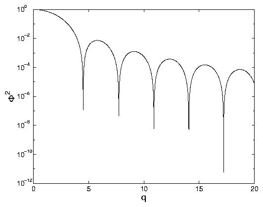
The intensity minima occur where F(x) = 0, that is, x = tanx. For large x, this approaches x = n p+ p/2. So, if many diffraction minima can be seen, their spacing will yield q R directly. The intensity maxima occur where dF/dx = 0, or

x2 sinx + 3 x cosx - 3 sinx = 0   .

(22)

The first zeros are at x = 0, 5.7635, 9.0950, 12.3229, 15.5146, 18.6890, 21.8539. For both minima and maxima, lim_{qR ® ¥} D(qR) = p. That is, qR is spaced by approximately p for all but the first few diffraction rings. The maxima for R corresponding to calibrants we have are listed in table

With this information, the peak minima or maxima can be fit to determine R. Or if R is known (in the case of a calibrant), then q can be determined. However, one important advantage of spherical calibrants is that the I(q) form has significance, unlike periodic calibrants, which can only provide a single length scale.

If there is any dispersity of radii, this will influence the intensity spectrum. Assuming a Gaussian distribution centered at x₀ with standard deviation s, the observed intensity is

I(q) = ó õ ¥ 0  dx  F2(x)  e-(x-x0)2/2s2

(23)

As discussed in references [3,], the intensity falls off as exp(-2 dq R). Because of the reciprocal nature of q and R, a spread in incident wavelength l will be indistinguishable from a spread in R. For this reason, the spherical calibrant data in this report were all acquired at CHESS where the the x-ray spectral width was narrow. Other effects, such as the size of the beam, will affect all modes equally and can be distinguished from the dispersion.

3.3  Software

The simplest calibration method is to determine the q spacing of peak maxima or minima far from the origin, as this value rapidly approaches p/ R as n increases. The next approach is to fit the minima/maxima positions, in analogy to the procedure for periodic calibrants. Here, the peak positions are not linear with q, but can be numerically determined from (22) or table 1.

3.3.1  TV6

With TV6, you can fit the intensity maxima, but not the entire lineshape. Begin ``finished'' image. That is it should be dezingered, background-subtracted, intensity-corrected, and distortion-corrected. For example, if your data images are dat1 and dat2 and backgrounds are bak1 and bak2:

>> move im1=dat1:dat2
>> move im2=bak1:bak2
>> move im3=im1-im2
>> move im4=im3!imi
>> move im5=im4!imd

This assumes that you have set the distortion correction images (with setdist) and intensity correction images (with setint).

Display your image with kut=0 (vary scal to taste):
>> disp im5 0 scal

Perform a dens with per-pixel normalization off; this enhances the weaker large-q peaks. Then, enter peak and edit the x-ray wavelength with x. Choose j to enter d-spacings. Pick values from table 2 corresponding to your calibrant. Then, choose c to calibrate and p. Now, TV6 will print z as the spec-to-phos distance in pixels. Unfortunately, it doesn't display a linear fit of d-spacing vs. pixel number, so the quality of the fit cannot be evaluated.

TV6 is now calibrated. Future fits in this TV6 session will use this value for z.

3.3.2  Matlab

[ Note: as of 2000-01-24, this may no longer be correct. The Matlab code is changing rapidly, and I haven't checked that this sequence of commands is correct. ]

The approach I take here is to fit the entire intensity profile.

To fit these in Matlab, load an rfile as described in section 2.2. To best see the intensity oscillations, choose Options -> Use Circles (off) and Options -> Y-axis: Porod Plot. Typically, the data near q = 0 may be overexposed and the data far from q = 0 will have a lot of noise and weak oscillations. To select only a portion of the data, choose Action -> Crop and select an range in x by clicking and dragging the mouse. (Only the x values are significant; the y-extent of the box is irrelevant.)

Now, choose Estimate and a box labeled qtgui:function will appear. Choose Spherical Calibrants and constant background. After the parameter box appears, you can enter parameters directly, or choose Function -> Estimate again from the main window. At this point, you can choose Function -> Fit and check if the parameters are close by comparing the line shapes. Otherwise, enter new values into the parameter edit boxes and either Action -> Redraw or re-fit.

If the fit is successful, then you know the mean mean radius in these arbitrary (pixel) units R_fit, as well as the true radius R_true. We also have

q Rtrue = p Rfit

(24)

so

z = 2 p l Rtrue Rfit

(25)

where z is in pixels.

Figure 5: Intensity maps of (a) Silica spheres (``synthetic rat''), (b) Polystyrene spheres (``ACF p.58-1 2A''). Because of the strong scattering near the center, there is significant streaking towards the right in both images. Azimuthal integrations were performed vertically (q = ±p/2 ±25^°).

Figure 6: Porod plots of (a) Silica spheres (``synthetic rat''), (b) Polystyrene spheres (``ACF p.58-1 2A''). These correspond to the images in figure 5.

4  Calibrant Inventory

All pre-made capillaries are in the top drawer of the first bench as you enter the wet room. These capillaries are detailed in table 3 below. Also in that drawer are materials for making spherical calibrant capillaries. In the dry box to the left are silver stearate and silver behenate.

calibrant	length scale (Å)	quantity	keyword
Ag-stearate	48.68	6	ACF Ag-ST 3 ¼7;
			MWT 3-5-98
Ag-behenate	58.376 ± 0.006	5	ACF Ag-BE 1 ¼5
silica spheres	278 ± 4	6	``synthetic rat'';
			ACF p.41-2 3A ¼ 3E
silica spheres	1360	5	ACF p.41-2 4A ¼ 4E
polystyrene spheres	250 ± 10	2	ACF p.58-1 1B;
			ACF p.131-1 1C
polystyrene spheres	1015 ± 22	6	ACF p.58-1 2A;
			ACF p.41-2 2A ¼ 2E

5  Cross-Calibrations

Cross calibrations are given in tables 4 and 5. These table were constructed by calibrating with the standard in the leftmost column and calculating the length scale (d-spacing or mean radius) of the other standards.

6  Acknowledgements

Thanks to Karen Edler for taking time out of her CHESS run and acquiring so many exposures on the spherical calibrants. This was a tedious job. Thanks also to Krysta Levac for supplying me with rat tails, and sparing me the most gruesome task. Rudolf Sprik kindly gave us the silica spheres, and Lois Pollack lent them to me.

7  Conclusion

If you notice any errors in this document or have trouble using/making calibrants, please let me know.

Adam C. Finnefrock

adam@bigbro.biophys.cornell.edu

References

[1]

T.C. Huang, H. Toraya, T.N. Blanton, and Y. Wu. X-ray powder diffraction analysis of silver behenate, a possible low-angle diffraction standard. Journal of Applied Crystallography, 26:180-4, April 1993.

[2]

T. N. Blanton, T.C. Huang, H. Toraya, C. R. Hubbard, S. B. Robie, D. Louër, H. E. Göbel, G. Will, R. Gilles, and T. Raferty. JCPDS - International Centre for Diffraction Data round robin study of silver behenate. A possible low-angle X-ray diffraction calibration standard. Powder Diffraction, 10(2):91-95, June 1995.

[3]

Mischa Megens, Carlos M. van Kats, Peter Bösecke, and Willem L. Vos. In Situ characterization of colloidal spheres by synchrotron small-angle x-ray scattering. Langmuir, 13(23):6120-6129, 1997.

[4]

Mischa Megens, Carlos M. van Kats, Peter Bösecke, and Willem L. Vos. Synchrotron small-angle X-ray scattering of colloids and photonic colloidal crystals. Journal of Applied Crystallography, 30:637-641, 1997.